Positional Embeddings

Hello readers, in our last blog, we learned about Token Embeddings and how they are actually implemented. Today, we will be extending that concept to generate embeddings for a whole sentence.

Okay, so what we learned about token embeddings is that they are meaningful n-dimensional projections of a single-dimensional token, i.e.:

word -> dog
token -> 13
embedding -> [0.14, 0.573, -0.345 .... ]

Now, let’s try to create embeddings or “projections” of a sentence itself, a.k.a. Sentence Embeddings.

Naive Approach

Let’s say you have a sentence

tom chase jerry

Now, how will you proceed if we want to generate the embedding of the whole sentence?

A naive way would be to take the average of all token embeddings, i.e.:

Let’s say we have 3-dimensional embeddings:

tom -> [0.2, 0.8, 0.4]
chase -> [0.5, 0.1, 0.2]
jerry -> [0.2, 0.2, 0.9]

Sentence embedding will be:

dim 1 -> (0.2 + 0.5 + 0.2) / 3 ->  0.3
dim 2 -> (0.8 + 0.1 + 0.2) / 3 -> 0.37
dim 3 -> (0.4 + 0.2 + 0.9) / 3 -> 0.5

tom chase jerry -> [0.3, 0.37, 0.5]

So, we were able to embed the whole sentence. Do you see any limitations in this approach?

Well, if you observe, the above method will generate the same embedding for:

 jerry chase tom

Why? Because we are taking the average of token embeddings. But as we saw, these sentences are not similar.

So, in our current approach, we are losing some information while generating the sentence embedding, i.e., in our embedding, we are not storing anything about the position of each token. That’s why it fails to distinguish the two sentences.

Positional Information#

So, we need to store the positional information as well in our sentence embedding.

A naive way to do so would be to just add their position index, i.e.:

position_aware_token_embedding = token_embedding + position

tom chase jerry

# adding 1,2,3 respectively depending on the word position

tom   -> [0.2, 0.8, 0.4] + [1, 1, 1]  = [1.2, 1.8, 1.4]
chase -> [0.5, 0.1, 0.2] + [2, 2, 2]  = [2.5, 2.1, 2.2]
jerry -> [0.2, 0.2, 0.9] + [3, 3, 3]  = [3.2, 3.2, 3.9]

tom chase jerry -> [2.3, 2.37, 2.5]

-----------------------------------------------------------

jerry chase tom

jerry -> [0.2, 0.2, 0.9] + [1, 1, 1] = [1.2, 1.2, 1.9]
chase -> [0.5, 0.1, 0.2] + [2, 2, 2] = [2.5, 2.1, 2.2]
tom   -> [0.2, 0.8, 0.4] + [3, 3, 3] = [3.2, 3.8, 3.4]

jerry chase tom -> [2.3, 2.37, 2.5]

Hmm, we still got the same embedding for both sentences, even though our token embeddings were different (since we added position).

Are we losing any other information that is resulting in the same embedding for both sentences?

Context Information#

Well, yes. Even though we added positional data, we didn’t store the “importance” of each token, i.e.:

Let’s assume in our vocabulary, “predator” holds high importance and “prey” holds low importance.

So, in our example, the first word (i.e., “predator”) has high importance, and the third word (i.e., “prey”) has low importance. But we didn’t store anything about it in our embedding.

Also, it’s quite possible that the same token at the same position might hold different importance in another example:

For instance,

tom was chased by jerry

Here, the first token denotes “prey,” i.e., low importance.

So, we observe that the same word “tom” at the same position “1” can have different importance depending on the context.

If I put this formally:

The projection/embedding of a token depends on its position and its environment.

So, instead of just “position-aware” embeddings, we want “context-aware” embeddings.

And to generate such embeddings, we need the “projection” of each token at different positions in different contexts or environments. And that is where the Self-Attention mechanism comes into the picture.

So, if we conclude, in our token embeddings, we also need to store:

• positional data, i.e., “positional embedding”
• environment data, i.e., “context-aware / attended embedding”

Today, we will be covering positional embeddings, and in the next blog, we will cover the Self-Attention mechanism.

Positional Embedding#

Okay, so how should we embed positional information in our token embeddings?

One way to do so, as we did earlier, is to add their positions:

tom chase jerry

# adding 1,2,3 respectively depending on the word position

tom   -> [0.2, 0.8, 0.4] + [1, 1, 1]  = [1.2, 1.8, 1.4]
chase -> [0.5, 0.1, 0.2] + [2, 2, 2]  = [2.5, 2.1, 2.2]
jerry -> [0.2, 0.2, 0.9] + [3, 3, 3]  = [3.2, 3.2, 3.9]

But there is a big limitation in this approach. Can you guess?

If you look carefully at the resulting embedding, the magnitude of positional information is much larger than the token embedding:

token embedding         [0.2, 0.8, 0.4] 
positional embedding    [1.2, 1.8, 1.4]

And this will further degrade for higher positions, say position 100:

positional embedding    [100.2, 100.8, 100.4]

Here, positional data dominates so much that it almost overshadows the actual meaning of the token. So any token at position 100 will almost have the same embedding. This defeats the purpose of embeddings.

tom   -> [0.2, 0.8, 0.4] + [100, 100, 100]  = [100.2, 100.8, 100.4]
jerry -> [0.2, 0.2, 0.9] + [100, 100, 100]  = [100.2, 100.2, 100.9]

Apart from this, we have 2 types of insights that can be extracted from positional information. They are-

• Absolute Position Insight
• Relative Distance Insight (also called Co-relation)

Absolute Position Insight

• Absolute Position helps to determine the depth of the token in the sentence, i.e., whether it’s present deep inside the context or at the start.
• Absolute Position has the following properties-UniquenessEach Position has a unique signature, for ex- index valuesOrderingThere is a notion of ordering among these values. For ex- if positions are denoted by index values, then a token at the start will have a smaller position value as compared to the one present much later
• UniquenessEach Position has a unique signature, for ex- index values
• Each Position has a unique signature, for ex- index values
• OrderingThere is a notion of ordering among these values. For ex- if positions are denoted by index values, then a token at the start will have a smaller position value as compared to the one present much later
• There is a notion of ordering among these values. For ex- if positions are denoted by index values, then a token at the start will have a smaller position value as compared to the one present much later

Relative Distance Insight / Co-relation

• Relative Position helps to determine the relation between 2 tokens, whether they are close to each other or far apart.
• Relative Position has the following properties:Position AgnosticRelative Distances are position agnostic. For ex- in case of index-based positions, the distance between 2 words is independent, regardless of where they are actually present. i.e., “tom chase jerry”, distance “tom” and “jerry” will always be 2, no matter where this chunk is presentOrderingThe relative distance values have a notion of ordering, i.e., in the case of index-based positions. The higher the distance, more far the tokens are and vice versa.
• Position AgnosticRelative Distances are position agnostic. For ex- in case of index-based positions, the distance between 2 words is independent, regardless of where they are actually present. i.e., “tom chase jerry”, distance “tom” and “jerry” will always be 2, no matter where this chunk is present
• Relative Distances are position agnostic. For ex- in case of index-based positions, the distance between 2 words is independent, regardless of where they are actually present. i.e., “tom chase jerry”, distance “tom” and “jerry” will always be 2, no matter where this chunk is present
• OrderingThe relative distance values have a notion of ordering, i.e., in the case of index-based positions. The higher the distance, more far the tokens are and vice versa.
• The relative distance values have a notion of ordering, i.e., in the case of index-based positions. The higher the distance, more far the tokens are and vice versa.

Hmm, so what we understand is that we have the following requirements for positional embedding:

• The magnitude of positional data should be normalized with respect to the actual embedding
• While normalizing, absolute positional information should not be lost
• While normalizing, correlationinsight should not be lost

This is where Sinusoidal Positional Embedding shines.

Sinusoidal Positional Embedding#

A sinusoidal wave is a simple oscillating curve defined by sine or cosine functions.

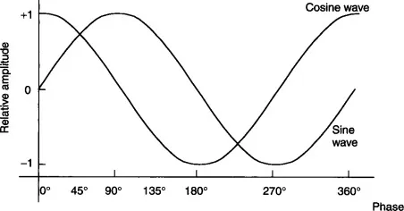
Sinusoidal Wave

So, as we know, the values of sine and cosine are always within the range [-1, 1]. This solves our first requirement: positional magnitude not overshadowing embedding magnitude.

But we had an additional requirement, i.e., preserving absolute positional information and correlation.

Let’s see how sinusoidal encoding handles this.

Sinusoidal World#

Each dimension in positional embedding is represented using sine/cosine functions of different frequencies:

pos(i) = [dim1, dim2, dim3, dim4 ..... dim n]

dim1 = cos(w1 * i)
dim2 = sin(w1 * i)
dim3 = cos(w2 * i)
dim4 = sin(w2 * i)
.......
.......

Note- The frequencies w1, w2, etc. occur in pairs, i.e., dim1 and dim2 are on the same frequency, dim3 and dim4 are on the same and so on… So if you have embedding of dimensions of 64, then there will be 32 different frequencies present.

For 4 dimensions:

pos(i) = [ cos(w1 * i), sin(w1 * i), cos(w2 * i), sin(w2 * i)]

pos(1) = [ cos(w1), sin(w1), cos(w2), sin(w2) ]
pos(2) = [ cos(w1 * 2), sin(w1 * 2), cos(w2 * 2), sin(w2 * 2) ]
pos(3) = [ cos(w1 * 3), sin(w1 * 3), cos(w2 * 3), sin(w2 * 3) ]
...........
...........
pos(i) = [ cos(w1 * i), sin(w1 * i), cos(w2 * i), sin(w2 * i) ]
pos(j) = [ cos(w1 * j), sin(w1 * j), cos(w2 * j), sin(w2 * j) ]

Absolute Positional Information

You might be wondering, why are we using different frequencies (w1, w2 …, etc.)

Why not use a single frequency? i.e.

pos(i) = [ cos(w1 * i), sin(w1 * i), cos(w1 * i), sin(w1 * i)]

As we know, sine and cosine are oscillating curves, i.e., they repeat their values after a 2π interval, so

pos(i + 2π) = pos(i)

which is incorrect, since it’s representing words at 2 different positions with the same positional embedding

Hence, we use multiple frequencies to provide a unique signature for each position, which is one of the properties of “absolute positional information.”

pos(i) = [ cos(w1 * i), sin(w1 * i), cos(w2 * i), sin(w2 * i)]

But there was another property, i.e., the notion of ordering, let’s see how we encode that

The frequency (w1, w2, w3 … ) is defined by the formula

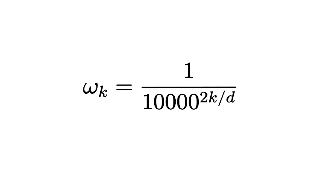
where d = “embedding dimension size”

If you substitute the values to derive frequency, then

w1 > w2 > w3 ....... wn

The higher the frequency, the higher the oscillation rate.

Let’s try to build some intuition around it.

Think of oscillation as moving around a circle. A higher frequency means you are running around the circle at a higher speed and vice versa.

Let’s say we are generating embeddings of 4 dimensions

dim1 -> w1 -> highest speed
dim2 -> w2 -> high speed
dim3 -> w3 -> medium speed
dim4 -> w4 -> low speed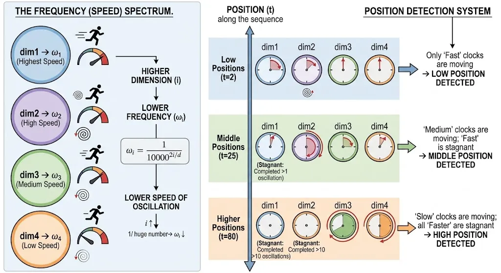

• For “lower” positions, dim1 and dim2 would have shifted by a lot , while dim3 and dim4 will be kind of stagnant

• For “middle” positions, dim2 and dim3 would have shifted a lot, while dim4 would have slightly shifted, and dim1 might be stagnant (it would have completed the whole oscillation)

• For “higher” positions, dim3 and dim4 would have shifted a lot, while dim1 and dim2 would be kind of stagnant (they would have completed their oscillation multiple times)

So, in this way, the absolute position, i.e., whether the position is far or close, can be detected by observing all the dimensions**.

Correlation Insight

Now, for calculating the correlation between 2 positions,

While using index-based positions, we used “subtraction” as the “mechanism” for computing correlation (calculating the distance between 2 positions)

In the case of a sinusoidal world, we use “dot product” as the “mechanism” for computing correlation, i.e.

rel(i, j) = pos(j) * pos(i)

Let’s substitute these values:

rel(i, j) = [ cos(w1 * j), sin(w1 * j), cos(w2 * j), sin(w2 * j) ] * [ cos(w1 * i), sin(w1 * i), cos(w2 * i), sin(w2 * i) ]

rel(i, j) = cos(w1 * j)cos(w1 * i) + sin(w1 * j)sin(w1 * i) + cos(w2 * j)cos(w2 * i) + sin(w2 * j)sin(w2 * i)

As per trigonometry:

cos(A - B) = CosACosB + SinASinB

If we substitute this in the above equation:

cos(w1 * j)cos(w1 * i) + sin(w1 * j)sin(w1 * i) = cos(w1 * j - w1 * i) = cos(w1(j - i))

cos(w2 * j)cos(w2 * i) + sin(w2 * j)sin(w2 * i) = cos(w2 * j - w2 * i) = cos(w2(j - i))

rel(i, j) = cos(w1(j - i)) + cos(w2(j - i))

Here, do you observe anything in our simplified correlation equation?

Well, it’s position agnostic, i.e.

rel(1, 3) = cos(w1(3 - 1)) + cos(w2(3 - 1)) = cos(w1 * 2) + cos(w2 * 2)

rel(17, 19) = cos(w1(19 - 17)) + cos(w2(19 - 17)) = cos(w1 * 2) + cos(w2 * 2)

So, we were able to achieve one of the properties required by correlation insight. Let’s see how we will bring the notion of ordering into it

When we were using index-based position, we had a notion that correlation would be larger for 2 distant positions compared to 2 closer positions, i.e.

rel(1, 3) < rel(1, 10)

In a sinusoidal world:

rel(i, j) = cos(w1(j - i)) + cos(w2(j - i)) + cos(w3(j - i)) ......

As discussed earlier, the frequency is defined by the formula:

And if we plot the “decay” rate for the above correlation function, we will notice that as the “relative distance” increases, the correlation value decreases, i.e., “closer” positioned words will have a high correlation value and vice-versa.

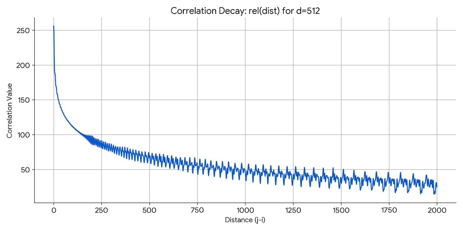
So, we were able to achieve a notion of ordering as well in the correlation.

Conclusion#

Today, we went a bit deep to understand why sinusoidal position embeddings are a perfect replacement for index-based positions, and how they store all information as provided by the latter.

If you look at the “Attention Is All You Need” research paper, the authors chose sinusoidal positional embeddings due to the same reasons.

Perfect! Our embedding contains positional data. And in the next blog, we will explore the famous “Self-Attention” mechanism and how it captures the meaning of a whole sentence by storing contextual information.

Stay Tuned..