Token Embeddings

Today, we will be covering another building block in our LLM series. I hope you have built a strong intuition around neural networks; if not, I would highly recommend reading my previous blog, Neural Networks, before proceeding.

Okay, so until now we have understood that any input we supply to an LLM or a model is converted into a numeric representation via Tokenization, and these numerics are then fed to a mathematical equation, a.k.a. a neural network.

Sample Neural Network as an equation:

 f(x1) = w1 * x1

If I increase the variables in this equation:

2 variables:
f(x1, x2) = w1 * x1 + w2 * x2

3 variables:
f(x1, x2, x3) = w1 * x1 + w2 * x2 + w3 * x3

n variables:
f(x1, x2, x3,..., xn) = w1 * x1 + w2 * x2 + w3 * x3 +....+ wn * xn

What advantage do you see in increasing the variables or “input dimension”, apart from giving you a headache :p

I hope you would have guessed that the greater the number of variables, the greater control we have to “fine-tune” so as to get the desired behavior, i.e., to understand complex patterns.

For example, via a single variable, you can only solve problems having a “linear” pattern. In real life, the patterns are quite complex, which requires multiple variables or “multi-dimensional” input.

If I go back to our tokenization blog, there we were able to map each token to its numeric representation of size or dimension “1”, i.e.:

Note*– For simplicity, I will be using “word”-level tokenization instead of “sub-word” level.*

Dataset:

Here comes the sun
Here comes the sun
And I say, "It's all right"
Sun, sun, sun, here it comes
Sun, sun, sun, here it comes

Post Tokenization:

Here  -> 0
comes -> 1
the   -> 2
sun   -> 3
...

So our tokenized input is of size 1, or formally, it is “single-dimensional” or “has a single feature.”

And as we saw previously, with a single dimension, we cannot derive complex patterns. For complex patterns, we need more “variables”, or “dimensions”, or “features.”

So, we aim to convert or “project” these single-dimensional inputs to their “n-dimensional” representations or “projections.”

Embeddings#

In a nutshell,

Embeddings are the “n” dimensional meaningful projection of a single dimensional input.

Here, notice that the projection needs to be “meaningful”. We will touch upon this later.

Core Idea#

Okay, since now we have understood what embeddings are and why they are needed, let’s explore the “how” part, i.e., how are these created/generated?

Let’s start from the basics. If I go back to high school mathematics, via which operation can we change projections?

I hope you remember, it’s via “matrix multiplication”. If not, no worries, let’s do a brief recap.

If I represent Matrix of dimension 'i' and 'j' as M[x, y]

then according to multiplication dimensionality rule:

M[i, k] * N[k, y] = O(x, y)

If we decrease the rank of the matrix to 1 for better understanding

M[1 * x] * P[x * y] = O(1 * y)

here P is also called "projection matrix"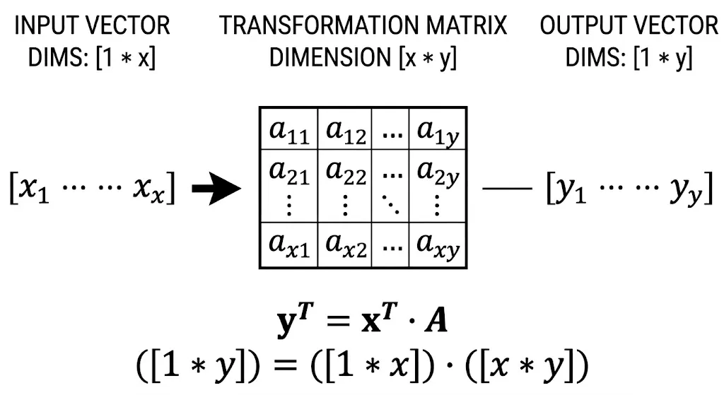

Matrix Projection

In simple words, if we multiply our input by the projection matrix, then our output will be of different (desired) dimensions. This is the core idea behind “embeddings.”

Now, since we know we will require matrix operations, we already know that matrix operations are an indirect translation of neural networks.

So now we know the tool via which we can create these embeddings, i.e., via neural networks.

Dataset Preparation#

What we studied about neural networks was that we train them on a dataset so that they can learn patterns by tuning the values of their weights via backpropagation.

So our target is to get a “trained embedding model” or a “learned matrix”. But how exactly can we quantify it as a task?

Our goal is to get a model that can “generate meaningful embeddings”, but we don’t have a dataset for which it can learn in a supervised fashion, i.e., we don’t have a dataset like:

word    |   expected_embedding
------------------------------
here    |    [1.0, 2.0, 3.0]
comes   |    [3.0, 4.0, 5.0]
............
............

In such scenarios, we follow a special paradigm in which we work on a “proxy” task or an “extended” problem, thereby indirectly training the required model.

Sounds confusing, right?

Note*– I’ll be referring to it as a “proxy” task instead of an “extended” problem.*

Let’s apply it to our problem statement:

Aim:

To train a model that can generate meaningful embeddings

Proxy Task:

To get a similarity score between two words

Now, if you think about this proxy task, how will you design the dataset?

We can think of a “typical” supervised training dataset like:

word1    |   word2    |  similarity_score
-------------------------------------------
dog      |    cat     |      0.79
lion     |    fish    |      0.21
...........................................
...........................................

But it’s extremely difficult to prepare such a dataset, isn’t it? i.e., how will you quantify the similarity scores that “dog” and “cat” are 79% similar, and so on

So, instead of following a “supervised” training approach, for such scenarios we do “unsupervised” training i.e. we train the model on a dataset with no pre-defined “scores” or “labels.”

So an unsupervised dataset for the above example will look like:

main word    |   similar words        |  non-similar words
-------------------------------------------------------------
dog          |    [cat, puppy]        |     [duck, eagle, lion]
lion         |    [tiger, cheetah]    |     [fish, shark, rat]
................................................................
................................................................

Now you might wonder how we create this dataset?

Well, the internet is filled with data. In a sentence, it’s a reasonable assumption that consecutive words are related.

Extending this, “k” neighboring words in a sentence can be considered similar, and far-away words as dissimilar.

This can be generated using a sliding window.

For example, let’s say you have a sentence

Dogs are loyal and playful while cats are independent and graceful

Note- As mentioned earlier, for simplicity, I’ll be using a word-level tokenizer instead of a “sub-word” level. So our vocabulary would look like-

Dog       - 0
and       - 1
Cat       - 2
beloved   - 3
pet       - 4
Loyal     - 5
Graceful  - 6
..........
........

And our dataset for this, with a window size of “3”, would look like-

main word      |    similar  word  |   non-similar word
---------------------------------------------------------
Dog            |    Loyal          |      Independent     
Cat            |    Indepednet     |         Loyal
......................................................
......................................................

Replacing it with their “numeric” labels based on their index in the vocabulary

main word      |    similar  word  |   non-similar word
---------------------------------------------------------
0              |    5              |      9     
2              |    9              |         5
......................................................
......................................................

Okay, so now our dataset is prepared, and we are ready to train for our “proxy” task

Training#

But how do we feed this to our neural network? As we saw earlier, with a single variable, our model can’t learn much pattern i.e., we cannot feed “cat” or “2” to the model. So we need to do some projection before we even start.

But wait, wasn’t it what we wanted to achieve, i.e., get an embedding model? Then how can we project our input if that is something we are expecting to derive?

So, if we go back to our definition of embeddings

“Embeddings are the n-dimensional meaningful projection of a single dimensional input.”

So while generating embeddings, our aim is to get projections that are meaningful in a way that they contain the properties of a given word with respect to multiple dimensions.

For example, if I have 2 words, “dog” and “lion”, and I want to project them in 3 dimensions

dimensions:
dim 0 - "are friendly"
dim 1 - "is carnivore"
dim 2 - "have 2 legs"

Now I project these 2 words on these dimensions:

dog  - 1 1 0
lion - 0 1 0

# dogs are friendly and carniovores but they have 4 legs
# lions are carnivores but they are not friendly and have 2 legs

So if we just look at the projections of “dog” and “lion”, these are meaningful in a way, i.e., via these projections we can interpret that 2 out of 3 dimensions are the same, so they are 66% similar. That is quite insightful!

Similar to this is what happens when we project embeddings to “n” dimensions. The only difference being you can’t quantify each dimension to some “human” understandable meaning as we do for “dog” and “lion.”

Okay, until now, we saw “meaningful” projections. We can also have”non-meaningful” projections as well.

Let’s say if I take the same example of “dog” and “lion”, and say if a vocabulary of size 5:

word    |    index
---------------------
cat     |      1
dog     |      2
penguin |      3
rabbit  |      4
lion    |      5

A non-meaningful projection for this would be their “index” positions i.e., we can have a projection of size equal to vocabulary with only the index bit set to 1, i.e.

cat   -  1 0 0 0 0      # 1st index bit set to 1
dog   -  0 1 0 0 0      # 2nd index bit set to 1
lion  -  0 0 0 0 1      # 5th index bit set to 1

So, as you see, we were able to project our words to a certain dimension, but do these contain any useful meaning? No, right, all these projections will be “orthogonal” to each other.

The above “non-meaningful” projection is also known as “one-hot” encoding, which is quite popular when you want to feed your input to a neural network whose only aim is to increase the variables/dimensions of our “initial” input.

So, once we generate the “one-hot” encodings, our input is of dimension “vocab-size”, which is quite large and enough

And now we have our input ready to be fed to a neural network.

Implementation#

Great, let’s start implementing what we learned so far..

Embedding Model:

• We define the neural network for our”model”, for now, it will just be a single-layer neural network Input dim = vocab size (one-hot encoding)Output dim = embedding dimension
• Input dim = vocab size (one-hot encoding)
• Output dim = embedding dimension
• In the forward loop, we are just computing the one-hot encoding and then supplying it to our model

import torch.nn as nn

class EmbeddingModel(nn.Module):
    def __init__(self, vocab_size: int, embed_dim: int):
        super().__init__()
        self.vocab_size = vocab_size
        self.model = nn.Sequential(
            nn.Linear(vocab_size, embed_dim, bias=False)
        ).to(DEVICE)
        nn.init.normal_(self.model[0].weight, mean=0.0, std=0.01)

    def forward(self, token):
        one_hot = F.one_hot(token, self.vocab_size).float()
        return self.model(one_hot)

Proxy Task:

• This is a bit interesting, our proxy task takes 3 params:center - which is the main wordpos_ctx - words which are similarneg_ctx - words which are not similar
• center - which is the main word
• pos_ctx - words which are similar
• neg_ctx - words which are not similar
• It returns the overall confidence score, denoting the main word is indeed similar to pos_ctx and not related to neg_ctx

class ProxyTask:

    def __init__(self, vocab_size: int, embed_dim: int):
        self.embedding_model  = EmbeddingModel(vocab_size, embed_dim)

    def execute(self, center, pos_ctx, neg_ctx):
        c = self.embedding_model(center)
        p = self.embedding_model(pos_ctx)
        n = self.embedding_model(neg_ctx)

        pos_dot = (c * p).sum(dim=1)
        neg_dot = (n * c.unsqueeze(1)).sum(dim=2)

        pos_conf = F.logsigmoid(pos_dot).mean()             
        neg_conf = F.logsigmoid(-neg_dot).sum(dim=1).mean()

        confidence = pos_conf + neg_conf
        return confidence

Initialization:

• We are aiming to generate embeddings of dimension 32, and we have a vocab size of 100

vocab = 100
EMBED_DIM = 32
EPOCHS = 25
proxy = ProxyTask(len(vocab), EMBED_DIM)

Backpropagation:

• So, as we saw, our “proxy” task returns a confidence score. Now, how will we backpropagate it i.e., we don’t have anything to compare it with, so how will we calculate loss?
• Well, it’s a bit counterintuitive; the task returns a confidence score. The higher the confidence, the better the model. So loss in this case will be the negation of confidence, i.e., low confidence -> high loss and vice versa, and that becomes our “loss function” based on which we will do backpropagation and run it through multiple epochs

optimizer = torch.optim.Adam(proxy.embedding_model.parameters(), lr=LR)

for epoch in range(EPOCHS):
    proxy.embedding_model.train()
    train_loss = 0.0
    for center, ctx, negs in train_loader:
        center, ctx, negs = center.to(DEVICE), ctx.to(DEVICE), negs.to(DEVICE)
        confidence = proxy.execute(center, ctx, negs)
        loss = -confidence
        optimizer.zero_grad()
        loss.backward()
        optimizer.step()
        train_loss += loss.item()

Inference:

• Once we have trained our model or the proxy task, we can simply extract the model and use it for our main purpose, i.e., to generate embeddings
• For ex- here the token 2 “represents” dog

model = proxy.embedding_model
token = 2
embeddings = model.forward(token)

Note:

To build intuition, I have skipped some of the internals and optimizations done to accommodate more non-linearities, efficiency improvements, and scalability concerns in real-world models.

Conclusion#

I hope you were able to build intuition around embeddings and how these models are trained.

In the next blog, we will take this a step further and learn how to generate embeddings for a whole sentence or context instead of just token-level embeddings. That is where the famous “Self-Attention” mechanism comes into play.

Stay tuned…